Assignment 6 is due at 2pm (before start of class) on Tuesday 4/27. Please see grading policy on course homepage for additional details regarding early/late submissions.

Please submit your answers in plain text (with any images as attachments) to i250hw@ischool.berkeley.edu.

---

1. Flow Control

Consider a GEO satellite channel that has a throughput capacity of 2Mbps. Assume that the satellite orbits at 20,000 miles above the earth, and that radio transmissions propagate at the speed of light. Assume that processing delays are negligible.

(a) (1 point) What is the round-trip-time (RTT) of this channel?

Speed of light, c = 186282.397 miles per second
RTT = 2*20,000/186282.397 = 0.215 second

(b) (1 point) If the stop-and-go technique is used for flow control, and the data packets are 1500 bytes in size, what is the maximum achievable data rate (in bits per second)?

With stop-and-go, we can send one packet per RTT, or 1500*8/0.215 = 55814 bits per second

(c) (1 point) Based on your answer to part b, what is the utilization of the channel capacity (in percent)?

Utilization = 55814/2000000 = 2.79%

(d) (1 point) If the flow control technique is changed to sliding window, what should the window size be so that the channel utilization is increased to at least 50%?

To increase utilization from 2.79% to 50%, which is a factor of 17.9, we need to increase the window size from 1 to 18 packets, or from 1500 bytes to 27000 bytes.

Note: This question is modified from Comer Exercise 26.7 (page 446).




2. TCP Congestion Control

A host transmits a VERY large file using TCP. 

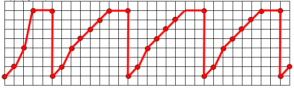
(a) (2 points) Assume that slow start and congestion avoidance are in force, but not fast retransmit, fast recovery, or flow control. Plot the size of the congestion window (cwnd) over time, starting with cwnd=1 at the beginning of the session.  Each horizontal grid represents one RTT, and each vertical grid represents one segment size.  Assume that the sender can send multiple segments instantaneously as allowed by the congestion window size. Further assume that, whenever cwnd reaches or exceeds 8 segments, the very next segment sent is lost (but not the subsequent segments), and the sender times out after 2 RTTs.

 

(b) (2 points) Assume each segment is 1000 bytes, and the average RTT is 100ms.  For the transfer of a very large file, what is the average throughput of this session (in bits per second)?

As we can see in the plot, after the initial session setup, the congestion window follows a regular pattern between timeouts.

Time between timeouts = 8*RTT

Number of segments transmitted during the 8*RTT cycle = 1 + 2 + 4 + 5 + 6 + 7 + 8 = 33 segments. However, one of the segments is lost, and has to be retransmitted after the timeout.

Therefore, average throughput = 32 segments * 1000 bytes/segment * 8 bits/byte / (8*0.1) seconds = 320,000 bps or 320 Kbps.

3. HTTP

Web browsers employ caching to improve access times of frequently requested pages. Section 4.8 of Comer describes caching in web browsers.

(a) (2 points) Describe the steps a browser takes to determine whether to use an item from its cache.

A browser saves the Last-Modified date information along with the cached copy. Before it uses a document from the local cache, a browser makes a HEAD request to the server and compares the Last-Modified date of the server’s copy to the Last-Modified date on the cached copy. If the cached version is stale, the browser issues a HTTP GET request to obtain an updated version from the server.

(b) (2 points) Look up the "conditional GET" method in the specification of HTTP/1.1. What advantage does this method offer over the HEAD and GET methods used in Algorithm 4.1 (page 58 of Comer)?

The use of the "conditional GET" method will avoid the extra RTT incurred in the event that the cached item is stale.

4. Multimedia Networking

(2 points) Explain how a jitter buffer permits the playback of an audio stream even if the Internet introduces jitter. [Comer Exercise 29.2, page 506]

The data packets for the audio stream, upon arrival at the receiver, are inserted into the jitter buffer, which is memory on the receiver's machine. Packets that arrive out of order can be reordered in the jitter buffer based on the timestamp information. The playback of the audio stream is based on reading of data from the jitter buffer at a constant rate, even though the data may arrive at the jitter buffer at a variable rate due to jitter. As long as the jitter buffer is not empty, the playback of the audio stream will not be disrupted. The probability of disruption can be reduced by introducing a delay between the transmission and the playback of the audio stream.